Playing with C++0x

The new C++0x standard (sometimes called C++11) provides new interesting features, like variadic templates and tuples. So, I’m experimenting a bit in order to test the technical requirements to put in practise the proposal for a new BTL, and I hit a problem of the GCC (I guess).

Proposal for a new version of the BTL

During the last months I have performed a job around the benchmarking tasks and I have gained a good knowledge of the Bench Template Library (BTL), which is a very good, generic, extensible, acccurate benchmarking library. However, I also found some problems that it has and seeked a solutions, at least ideally. In this document I will explain these and present a project for renewing the BTL.

When I cite the BTL in this document, I refer to the current version in the eigen mercurial repository.

Foundations of the BTL

The BTL is based upon interfaces to many numerical libraries. These are classes that wrap the calls to the library functions. The idea is the same as for the abstract classes-inheritance paradigm, but in this case C++ templates are used and the wrapper methods are usually inlined, which makes this system being very reliable for the benchmarking purposes.

Besides, a set of actions is defined. An action is a class that acts on an interface for performing a particular numerical job with a specific size. For example, there is an action for the axpy operation, one for the triangular system solver, one for the matrix-vector product. Each action has the following public methods:

• A constructor which takes the problem size as integer; this creates the needed generic matrices and vectors, and copies them to the interface-specific objects.
• An invalidated copy-constructor.
• A destructor which frees the memory.
• name which returns the name of the action as std::string (along with the interface name).
• nb_op_base which returns the number of base (floating point) operations performed by the action.
• initialize which performs some preliminary task before computing the result. This is in theory useful for libraries (e.g. BLAS) that do in-place computations; then this method regenerates the input data.
• calculate which performs the actual computation.
• check_result which implements a basic check for the output of the computation; in case of failure exits the program with an error message and code.

All actions take as class template parameter an interface.

The real BTL code resides in the generic_bench directory, where a set of utilities and other generic functions are defined. The utilities allow the actions to construct random matrices, vectors. The function bench and the PerfAnalyzerclasses are the real core of the BTL and perform a great job.

Now, for each library that has to benchmarked a program has to be compiled, linked and executed. The program is based upon main.cpp files that are delivered along with the interface – the main.cpp is slightly interface-dependant – and has compile instructions by means of the CMake tool.

Drawbacks of the BTL

I will now point out some problems that I found on the BTL during my work:

• Input data. For the benchmarks to be unbiased, all interfaces have to be in the same situation when doing a job; this includes the input matrices and vectors. Basic linear algebra algorithms like matrix-vector multiplication or vector sum usually do exactly the same job on any input data; but more complex algorithms, like sparse solvers, have a run time and an amount of floating point operations that strongly depends on the input data. For example, the Conjugate Gradient Method could need a strongly different amount of iteration when applied to two equally-sized slightly different matrices and starting vectors. This is the reason because a different, more evolved way to construct random matrices has to be considered. We will do this by means of a deterministic random number generator. In other words, the input matrices construction has to be reproducible.
• Results representation. In the current version, the benchmarking results are represented by means of megaflops (milions of floating point operations per second). This is a common way to represent results, useful and handy, but sometimes wrong. One of the objectives of the BTL, at least in my opinion, is to be generic. The design of the library, the implementation of the core functions is actually a very good starting point for a really generic benchmarking library; in my project I could add FFTW, distributed-memory benchmarks by just adding interfaces, actions and with few changes to the core library. The action-specific number of base operations is not very generic, in facts. Two different libraries can use different algorithms to solve the same problem, resulting in a different amount of floating point operations; the number of operation could depend on the input data (e.g. for sparse algorithm this s often the case); it could strongly depend on the size of problem, as for the FFT, where the algorithms can be more or less optimized depending on whether the size is a product of small prime numbers or not. Each of these (quite common for non-basic tasks) lead to situations where the action class can not correctly determine the number of floating point operations involved in the calculation, resulting in benchmarking outputs that are useful to compare different libraries, but basically wrong. Some consideration will be done to solve this issue.
• The Bench Template Library is not a library. This is not a real problem, but some meditation can be done in this field, though. A library is defined as a set of classes and functions (and objects, macros and other entities) that are used in other programs. The BTL is actually a library and a set of program sources and a set of compile an run instructions. It could be possible to design a real library with some function that would perform the benchmarks of different libraries and provide the results by means of a predefined interface (directly to file or as return value of a function); this library could be used in a program independently of the compile instructions. This lead to some problems, some of them are solvable and are treated below.
• Mixed use of the STL. The BTL makes sometimes use of the STL objects, and relies some other time on new/delete operations. This is not a problem for the current version of BTL, but make things slightly more difficult for the reader or the programmer that wants to extend the BTL, for instance adding new actions. My proposal is to make a more extensive use of the STL, in particular of the vector template class, in order to simplify some operations and definitively avoid memory leaks. The new C++0x syntax (and many standard C++98 compilers with some advanced optimization) also avoid copy-construction of vectors when not needed – move construction –, resulting in a easier, less error-prone and equally performing and memory using programming paradigm.
• Initialize. Some attention should be payed regarding the initialize and calculate methods of the actions. The initialize method should prepare the input structures for the calculate operation. This means that initialize should be always called before calculate. This is not the case, at least in the current version: initialize is called, then calculate is called many times (such that the measured time is at least 0.2 seconds). In case of an in-place operation, this is a problem. Consider the cholesky decomposition: a symmetric, positive definite matrix A is constructed and a copy of it is called A_ref; the calculate method calls the library function that reads A and writes the resulting L matrix into the same memory location of A; this leads to the situation where A is not an SPD matrix anymore: A_ref should be copied into A and the computation could be then performed again. Now two – interconnected – reflections have to be done. Firstly: the time required by initialize should probably not be taken into account for the benchmarking process; this would require that the timer just measures one execution of calculate, then stops, avoiding the benefits of the current measurement process, which lets the timer measure the time required by many runs; as result, the benchmark could not be accurate for small sizes. Secondly: not-in-place implementations do not present such problems, probably because they internally perform similar copy operations; therefore some attention has to be taken when considering the difference between in-place and not-in-place implementations. Lastly, some strict rules have to be defined in order to be completely unambiguous with respect to the content of both functions (which operations are allowed to be placed in initialize and not be benchmarked, which are restricted to calculate).
• Checking the result. As said, the action itself checks the results and, in case of failure, exits the program. Well, this sound a naive behavior: in case of an error an exception should be thrown, or, in case we want to avoid the usage of C++ exceptions – so think I –, a false value should be returned by the check method and the BTL itself (not each action separately) should take the decision on what to do, how to notice the error to the user and how to continue the benchmarks.
• More flexibility. As improvement of the BTL, some other usage cases could be considered. As stated before, I adapted the BTL to also support distributed-memory libraries (ScaLAPACK). In order to do things well, some more internal change could be considered, in order to make the BTL even more generic.

In the following I will propose some possible solutions for the problems that I pointed out. Let’s start with the more challenging points.

How to benchmark different interfaces together

In the current version of the BTL, the bench function takes as template parameter an action, which in turn takes as template parameter an interface. Instead of doing so, we could imagine a new bench function, which makes use of variadic template arguments and tuples – introduced in the C++0x standard, which is now supported in many C++ compilers: the first set of arguments (the first tuple, but this definition would not be exact; better: the first tuple specialization) would describe the interfaces, while the second one the actions.

typedef std::tuple <
  eigen3_interface,
  blitz_interface,
  ublas_interface
> interfaces_tuple;

typedef std::tuple <
  action_axpy,
  action_matrix_vector_product,
  action_cholesky_decomposition
> actions_tuple;

int main()
{
  bench<interfaces_tuple, actions_tuple>(/* arguments of bench */);
}

Then, bench would iterate over actions, then over interfaces and generate all possible combinations. Benchmarking all the interfaces together with respect to a specific action would solve some problems; for instance, this would aid to avoid too long benchmark run times, keeping the accuracy of the results as high as possible.

Now, there is a problem with libraries that have the same interface. The most important example is BLAS: BLAS is a stadardized interface with a reference implementation written in Fortran and other optimized implementation written in Fortran, C or C++ with the same interface; depending on the library the executable is linked with, the desired implementation is chosen, and with this method it is impossible to run two different BLAS implementations in the same execution. There is a solution: load the desired library at run time. Consider the following class:

class BLAS_interface
{
public:
  BLAS_interface(const std::string& library) {
    void *handle = dlopen(library.c_str(), RTLD_NOW);
    if (!handle)
    	std::cerr << "Failed loading " << library << "\n";

    axpy_func = reinterpret_cast(dlsym(handle, "daxpy_"));
    char *error;
    if ((error = dlerror()) != NULL)
    	std::cerr << error << "\n";
  }

  // C++-friendly axpy interface : y   void axpy(
    const double& alpha,
    const std::vector& x,
    std::vector& y
  ) {
  	const int N = x.size();
  	const int iONE = 1;
  	axpy_func(&N, &alpha, &x[0], &iONE, &y[0], &iONE);
  }

private:
  typedef void (*axpy_t)(const int*, const double*, const double*, const int*, double*, const int*);
  axpy_t axpy_func;
};

This solves the problem of having different libraries with the same interface. But a new issue arise: until now the interfaces did not need to be instantiated: the methods were static and no property was saved; with this version one has to instantiate an object of the BLAS_interface class and use that object to call the functions. Therefore, a template parameter is not sufficient anymore to define an interface, but an actual object is needed. This is not a problem, but we have to clearly state that the interfaces are not anymore static classes, but have to be instantiated. Nothing forbids them to be signleton classes, which would actually be a sensible design pattern to implement for the interfaces that do not need an external linked library, or that only have one possible external library.

There is still a point that could be taken into account: what about interfaces that load an external library that in turn load another external library? This seems an exotic situation, but in facts it is a common one: usually LAPACK implementation rely on a BLAS implementation for the basic operations. Is it possible to benchmark separately the LAPACK reference implementation when using the openblas BLAS implementation and the same LAPACK implementation when using the ATLAS BLAS implementation? Yes, it is possible, but requires some changes to the simple framework that I just presented.

When opening an external shared library, one can add the option RTLD_GLOBAL, which means that the symbols are made available to all successively opened shared libraries. By the way, doing so with a BLAS library is necessary to open a LAPACK library. This is where we can choose the BLAS implementation to use with a specific LAPACK implementation. The only problem is that we have to close both BLAS implementation and LAPACK implementation shared object files if we want to chage BLAS implementation. Therefore I propose the following: each interface, along with the computation methods, has two more methods: prepare and clean. They are called just before the call to any computation methods and just after, and at each time there is only one (or zero) interfaces that is prepared. For most interfaces both methods can be void, while for LAPACK interfaces, or any other implementation with a library that has dependencies that we want to manage, it could be something like this:

class LAPACK_interface
{
public:
	LAPACK_interface (const std::string& blas, const std::string& lapack)
		: blas_(blas), lapack_(lapack)
	{ }

	void prepare() {
		handleBLAS = dlopen(blas_.c_str(), RTLD_NOW | RTLD_GLOBAL);
		handleLAPACK = dlopen(lapack_.c_str(), RTLD_NOW);

		dgesv_func = reinterpret_cast(dlsym(handleLAPACK, "dgesv_"));
	}

	void clean() {
		dlclose(handleLAPACK);
		dlclose(handleBLAS);
	}

  // C++-friendly dgesv interface : B   // Matrix storage is column-major
  // Returns the pivots and changes B
  std::vector solve_general(
    const std::vector& A,
    std::vector& B
  ) {
  	const int N = std::sqrt(A.size());
  	const int NRHS = B.size() / N;
  	std::vector ipiv(N);
  	int info;
  	dgesv_func(&N, &NRHS, &A[0], &N, &ipiv[0], &B[0], &N, &info);
        return ipiv;
  }

private:
	typedef void (*dgesv_t)(const int*, const int*, const double*, const int*, int*, double*, const int*, int*);

	const string blas_, lapack_;
	void *handleBLAS, *handleLAPACK;
	dgesv_t dgesv_func;
};

The new algorithm

All interfaces will be tested at the same time, which requires a new algorithm for the benchmarks. Briefly, testing all the interfaces doing an action of a given size is splitted into two stages.

The first stage determines how many times the calculation has to be run in order to make an unbiased and accurate benchmark. The BTL will pick a seed, generate the corresponding input matrices and loop over the interfaces: for each interface, the input is set, the the timer measure the time required for running the computation. This is done for many seeds and for each interface the times are summed, until the slowest interface reaches a given total time. The number of tested seeds is called “maxseed” and these will be the same seeds for the second stage. The slowest interface will run them once, while the other will run them as many times as the ratio between the time required by the slowest interface and them.

In the second stage the benchmarks are run the computed number of times, separately for each interface, with the same seeds as in the first stage.

As understanding my explanation is quite difficult, I make an example. Imagine we have three interfaces I1, I2 and I3 and want to test them for the action matrix-matrix-product with 300-by-300 matrices. We start with the seed 0 and generate the set of input matrices with this seed. Then we let interface work with these matrices and measure the time required — e.g. I1 requires 0.3 seconds, I2 lasts 0.9 seconds and I3 0.4 seconds. The we start with a new seed (i.e. 1) and do the same; we sum the results for each interface and have now the values 0.6, 1.7, 0.8. Say our stop time is 2 seconds, then we have to run the computation (at least) another time with a different seed. Now we pick the seed 2 and after the computation we have the following values: I1 -> 0.9 sec, I2 -> 2.7 sec and I3 -> 1.3 sec — and we stop because the slowest interface (I2) reached the 2 seconds limit. This means that the first interface is approximately three times as fast as the second one and I3 is twice as fast as I2.

During the second stage we pick the first interface, iterate over the seeds 0..2 and for each seed we let the interface compute three times the result and finally average the result. We do the same with the interface I2, but this time we let it compute the result just once for each seed. I3 will compute the result twice for each seed. Eventually, the average for each interface is stored as result. Optionally, we could run the second stage more than once. The current BTL acutally has a similar algorithm and runs this second stage 3 times — this value is customizable.

How to generate and store matrices

The BTL decided to store matrices as STL vectors of vectors. This method makes it easy to read and write the matrix using the indices and allows the direct retrieval of the number of rows and columns. As drawback, it is slightly difficult to sequentially read or write the matrix, with either a row-major or column-major strategy. I would prefer this second need and store therefore the matrices just as long vectors, using a lexicografic ordering, and more precisely the column-storage strategy, which seems to be the most used one. As the actions are responsible for the generation of matrices, they also know these pieces of information and will not have problems when computing things — or delegating the computation to the interfaces — with the matrices. The same strategy can apply to N-dimensional arrays, which are useful in some tasks, like FFT.

The generation of a matrix is governed by the shape of the matrix and a seed, which is an integer. The seed is the initial value for a deterministic random number generator. A very simple yet powerful one is the linear congruential random number generator. The matrix generator would take a shape (specialization/overloads will be present for vector and matrices) and a seed and return an std::vector with random entries representing a vector, matrix or more-dimensional array. Notice that the new move syntax in the C++0x standard will avoid useless and expensive copies.

The last paragraph presented the most simple case, i.e. dense, random matrices. In case of symmetric matrices, only the upper part is generated, and the lower part is just copied from there. The same strategy will be used for SPD matrices, but to the result will be added the value N·maxv to the diagonal, where maxv is the absolute value of the maximal possible entry in the matrix (i.e. the maximal value returned by the random number generator).

How to represent and store the results

In my opinion, the benchmarking library should just measure as good as possible the performance of a library, i.e. the time is spent for a computation operation. It should not see to the representation of this data. Therefore, the output of a benchmarking library should  just be the time in seconds. Then, while representing the data could decide to plot the time against the problem size or try to retrieve the number of floating point required by one operation and plot the MFlops against problem size, this does not matter for the BTL. Therefore, I would save into the files just the sizes and the seconds.

Now I make a short excursus on how to plot the data. I see three possibilities:

• Time vs. Size. Has many drawbacks. The only sensible possibility seems a loglog plot, because a semilogx plot would make it impossible to distinguish the time required by small sizes and a linear x axis would collapse this information into the left part. The loglog could be useful to understand the time-complexity of the algorithm, but is not very useful to compare different libraries.
• MFlops vs. Size. This is the most used plot and has many advantages. It solves the issues of time vs. size, but has the drawback that I already explained: it can be wrong.
• Time vs. Size with respect to a reference result. In this plot, a reference implementation is picked and its result is displayed as straight line with value 1; the time required by the other imlementations is displayed as fraction of the time required by the reference implementation. Provided that the differences between the reference results and the other are not too big, this plot combine the benefits of boths methods. A semilogx would be a reasonable strategy for the axes.

Now a few remarks on how to store the data. BTL now writes one file for each tested library and each action, and this files contains two columns: one for the sizes, one for the results (in MFlops). This makes the information redundant — if we want to test the same sizes on all libraries –, since the sizes is written many times. I would instead place all libraries for a given action in the same file, which makes it easyer to read and compare them, takes less space and is a more clean way to save files. Moreover, dat files have some drawbacks, which made me create a C++ library for handling MAT files as bachelor thesis. MAT file are the standard used by Matlab for storing data, can store more than one matrix, support named arrays, stores the data in binary form, occupy less space than DAT files and are an open standard, which does not require external tools but the Zlib. I propose the following structure for a BTL file:

• The header can contain some information: here we would add the name of the action.
• The first array would contain the sizes (integer array). Its name would be sizes.
• The second array would contain the number of seeds used for each size. Its name would be seeds.
• Then, all libraries would have an array with the time in seconds, whos name would be the name of the library.

This would allow the BTL adding libraries to the file at a later time in a very consistent way, doing exactly the same tests as for the other libraries. It could be also possible to add an array mapping array names to library descriptions in order to generate more user-friendly graphs. Notice that Matla, Octave, Numpy and other widely used numerical software can handle MAT files.

The example continues

Yesterday we have seen how can we scatter a matrix which resides on a core among the processes. Now I want to make the code clearer and encapsulate it into a function. I call the function dscatter and the following are the parameters:

• const int& context: input, the blacs context
• const double* const& GlobalMatrix: input, only relevant for the root process; for the other processes it is safe to use a random pointer or NULL
• double*& LocalMatrix: output, the given pointer is useless; a new one will be stored there; an allocation will be performed, so after the execution the user has to free the memory using delete[].
• int& GlobalRows: input for root, output for the other processes; after the execution contains the global number of rows
• int& GlobalCols: input for root, output for the other processes; after the execution contains the global number of columns
• int& BlockRows: input for root, output for the other processes; after the execution contains the number of rows in each block
• int& BlockCols: input for root, output for the other processes; after the execution contains the number of columns in each block
• int& LocalRows: output, after the execution contains the number of rows of the local matrix
• int& LocalCols: output, after the execution contains the number of columns of the local matrix
• const int& root: input, the BLACS id of the matrix that owns the global matrix.

An example of BLACS with C++

I’m shocked by the lack of examples or guides on the web regarding BLACS, PBLAS and ScaLAPACK. Therefore, I decided to post here some examples. Many people (and I among them) use the C or C++ language instead of Fortran and therefore need a way for accessing the Fortran routines from there — not so difficult: the function arguments are always pointers, the function names are usually in lower case and with a trialing underscore — or have a more comfortable C interface.

In this example I will load a matrix from a file into the root process, scatter it among the processes according to the block-cyclic pattern, print the local matrices, then gather the local matrices onto the root process and control that the original matrix and the gathered matrix are the same. I will use for that MPI, BLACS with its C interface and some helping routine from ScaLAPACK (just numroc).

Before I begin with the example, two remarks:

• The example is useful for explanatory purposes, but is in facts not so useful in the real-life work: most often we use distributed memory programming because the data would not fit into a single computer memory. For instance, if we want to make a computation that involves a 500,000-by-500,000 matrix of doubles, this would sum up to 250,000,000,000 doubles, which results in 2,000,000,000,000 bytes = 2 TB. There is no single computer with such a memory (as far as I know…). Therefore it makes no sense to load the whole matrix into the root process. But we will most probably test tiny matrices, so forget this for now.
• If you landed here and decide to continue reading, PLEASE, let a message in the comments. Critics, suggestions, comments are very welcome.

You can find the official documentation of BLACS on netlib:

• The reference to the routines
• The quick reference to the C interface
• Some papers

It is not always very clear, but once you made yourself familiar with BLACS, it is a good quick reference.

You will find more examples in the Parallel Computiung category on this blog. Stay tuned, if you are interested!

Compilare Koffice

Nel pieno della compilazione

Pochi giorni fa è uscita la versione 2.2 di Koffice. Mi ha sempre entusiasmato, e quindi deluso, questa suite che si propone come alternativa a… A che cosa? A Office o a OpenOffice.org? Forse a entrambe.

Devo dire che, quanto a originalità, questo progetto non ha mai peccato, sia come interfaccia grafica che come funzionalità. Ma a dire la verità non sono mai riuscito a sentirmi a mio agio dentro la finestra di questi programmi. Spero che prima o poi riuscirò a vincere questa situazione, perché, per quelle poche volte che ho bisogno di uno strumento d’ufficio, vorrei avere dei programmi ben integrati e soprattutto un po’ più reattivi di OpenOffice, che a volte mi fa proprio imbestialire.

Mentre mi si sta compilando, ne parlo un po’ qui, tanto per passare il tempo.

Matlab: pubblicare funzioni

La finestra dell'editor

Abbiamo appena finito di scrivere la nostra funzione che, dati n parametri in input, calcola qualcosa, magari fa qualche grafico e dà m valori in output. Vogliamo ora pubblicare questo file in maniera almeno un po’ professionale, in modo che il codice sia leggibile, i risultati per un dato input chiari e i grafici visibili.

Matlab ci mette a disposizione alcuni strumenti semplici e utili. Dall’editor possiamo scegliere il pulsante publish, accanto al tasto per la stampa per pubblicare in formato html il file con la funzione e gli eventuali risultati.

Se la nostra funzione prende in input alcuni argomenti e non esistono clausole interne per standardizzare gli argomenti non dati, o semplicemente vogliamo che la funzione venga richiamata in un determinato modo, possiamo variare il modo in cui viene richiamata tramite il pulsante Edit Publish Configurations, presente nel menu che si apre selezionando il pulsante citato. Nella finestra che si apre possiamo impostare vari tipi di pubblicazione, diversi output, varie configurazioni di lancio, la directory in cui salvare i file e via dicendo.

Tra li altri possono essere scelti i formati html, pdf e latex; si può scegliere in che formato esportare le immagini, in che modo catturarle, se includere tutto il codice e se evidenziare anche gli eventuali errori. Tutto ciò nella sezione inferiore. Nella sezione superiore, invece si può inserire il codice di lancio della funzione o del file. Nel mio caso, per esempio, carico un file contenente alcune variabili e richiamo la funzione dando alcune di queste variabili in input, richiedendo invece l’output nelle tre variabili a, b e c.

La finestra di configurazione

Le configurazioni elencate a sinistra (nel mio una sola) possono essere di pubblicazione (come questa) o di lancio, per la quale ovviamente tutte le opzioni riguardanti la pubblicazione non vengono date. Configurazioni di lancio sono usate quando l’utente richiede il lancio di un file senza richiamare direttamente la funzione da una finestra di comando. Anche queste possono rivelarsi molto utili quando si vuole che l’utente possa eseguire la funzione piuttosto che dargli un rapporto già fatto dei risultati.

Bisogno urgente di RAM?

Non parlo di costosa memoria RAM fisica, ma di spazio da usare come memoria volatile, anche se volatile non è. Chiarisco: si tratta di swap, ossia di una parte – di dimensione arbitraria – di hard-disk che viene usata come estensione della memoria di lavoro a disposizione del computer. In genere tutti coloro che si affacciano sul mondo linux e che quindi hanno a che fare almeno con un’installazione – fosse anche la semplicissima procedura di Ubuntu – hanno acquisito il concetto di swap come partizione supplementare che non contiene dati stabili, ma che viene trattata dal sistema operativo come memoria ad accesso casuale. Ma lo swap non è solo questo. Altri sistemi operativi hanno previsto l’esistenza di swap senza una partizione dedicata, ma all’interno di un unico file. E GNU-Linux permette anche questo tipo di swap, che si rivela particolarmente utile in situazioni nelle quali un unico compito richiede molta più memoria di quella a cui il sistema sia abituato. Se ci stiamo imbarcando in un’impresa computazionale che richiede una quantità inusuale di memoria RAM e non abbiamo previsto per questo tipo di operazioni una partizione a parte, impiegheremo circa 30 secondi (o poco più a dipendenza della dimensione necessitata e della velocità di scrittura dell’hard-disk) e pochissimi semplici comandi per procurarcela.

Plot tridimensionali con Matlab (o Octave)

Un (brutto) grafico tridimensionale

Mi riferisco alla funzione mesh. E non voglio in alcun modo essere esaustivo; per una documentazione esaustiva, quella di Matlab lo è di sicuro.

Ammettiamo di voler fare il grafico della funzione .  La prima cosa da fare è generare la griglia. Come nel plot bidimensionale, in cui la griglia è unidimensionale ed è quindi un semplice vettore contenete le componenti delle ascisse in cui il grafico viene mostrato, nel caso tridimensionale avremo non un solo vettore, ma due matrici: ogni componente di ciascuna matrice rappresenta un punto del piano di base (piano xy) in cui il grafico viene calcolato e la prima matrice rappresenta il valore della x in quel punto, mentre la seconda rappresenta il valore della y. Si veda pertanto il seguente esempio per comprendere il significato di questa coppia di matrici.

Con queste matrici si ottiene una griglia che contiene i seguenti punti:

• (1, 4): primo elemento della prima riga di ogni matrice
• (2, 4): secondo elemento della prima riga
• (1, 5): primo elemento della seconda riga
• (2, 5): secondo elemento della seconda riga

Fatto ciò, si deve solo definire una matrice Z, della stessa dimensione delle matrici X e Y, che contenga i valori della funzione nei punti definiti tramite X e Y. Nel nostro esempio, il la matrice Z dovrà contenere:

• 2 nel primo elemento della prima riga ()
• 8 nel secondo elemento della prima riga
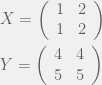
• nel primo elemento della seconda riga
• nel secondo elemento della seconda riga

Ora basterà richiamare la funzione mesh di Matlab per avere un meraviglioso grafico della nostra funzione. Per la precisione, la funzione va richiamata così: mesh(X, Y, Z), dove X, Y, Z sono le tre matrici che abbiamo definito.

Ora, per fare un grafico, ovviamente, sono necessari più di quattro punti per la griglia. La funzione meshgrid può venirci in aiuto: dati i vettori di x e di y (nel nostro caso i vettori erano (1, 2) per x e (4, 5) per y), la funzione meshgrid(x, y) restituisce le due matrici X e Y che costruiscono la griglia. Si veda il seguente esempio:

x = -4:0.1:4;
y = 0:0.1:5;
[X, Y] = meshgrid(x, y);
Z = X.^2 .* sqrt(Y);
mesh(X, Y, Z);

Ovviamente il grafico deve ancora essere corredato di un titolo (funzione title), di etichette per gli assi (funzioni xlabel, ylabel e zlabel) ed eventualmente di altri accorgimenti. L’importante è notare la semplicità di usare funzioni e operatori component-wise per generare la matrice Z: in una sola e semplice riga di codice si ottengono tutti i (molti) valori necessari.

Geometria interattiva con Kig

Uno strumento di kdeedu che mi sembra davvero ottimo per lo studio della geometria è Kig. Questo programma offre un’enorme varietà di strumenti per la costruzione di lavori di geometria planare e può risultare utile non solo a studenti delle scuole medie o medie superiori, ma anche a utenti più esperti.

Le entità geometriche con cui si può lavorare variano dai semplici oggetti che tutti conoscono (rette, semirette, segmenti, vettori, circonferenze, ellissi, parabole, coniche in generale, poligoni,…) fino a trasformazioni che non sono proprio alla portata di tutti (dalle semplici traslazioni o rotazioni fino a trasformazioni proiettive).

Naturalmente, il punto di partenza di tutto è il punto, che può essere piazzato sul foglio di lavoro con il mouse oppure dandone le coordinate cartesiane esatte.

Costruzione della circonferenza

Qualche esperimento tra Sabayon e Gentoo

È da un po’ che ho voglia di provare a costruire un sistema Sabayon Core – Gentoo, nel senso di partire da una Sabayon Core “pulita pulita” e trattarla come se fosse una Gentoo “già iniziata”, ossia installare Sabayon Core, aggiornare i pacchetti già installati tramite entropy e da lì in avanti usare soltanto portage per compilare tutto il resto del sistema.

Il primo esperimento in questo senso lo sto conducendo in questi giorni, molto rozzo, su una macchina virtuale (con VirtualBox). Per il momento non va male. Ho installato Sabayon Core, aggiornato il sistema con equo, poi aggiornato l’albero di portage (layman compreso) e dato un “emerge -uD world”; questo ha causato l’emersione di 101 pacchetti, l’ultimo dei quali, l’upgrade di gcc dalla versione 4.4.1 alla 4.4.2, ha restituito un errore. Suppongo si tratti di una problema temporaneo, causato dai grandi cambiamenti che gli altri 100 pacchetti hanno apportato al sistema. Appena avrò un minuto riavvierò la macchina, darò una controllatina alla configurazione e riproverò.

Spero che questi miei esperimenti possano diventare interessanti quando avrò il sistema pronto ad accogliere un’installazione di KDE. Si capirà la bontà di Sabayon, soprattutto della versione Core, come sostituzione della laboriosa installazione di Gentoo.